Next: GBT Active Optics Systems and Techniques
Up: Adaptive and Active Optics
Previous: Adaptive and Active Optics
Table of Contents -
Subject Index -
Author Index -
PS reprint -
Véran, J.-P. & Durand, D. 2000, in ASP Conf. Ser., Vol. 216, Astronomical Data
Analysis Software and Systems IX, eds. N. Manset, C. Veillet, D. Crabtree (San Francisco: ASP), 345
Reduction of Adaptive Optics Images
J.-P. Véran
National Research Council, Herzberg Institute of Astrophysics, 5071 West Saanich Road, Victoria, B.C. V8X 4M6, Canada
D. Durand
National Research Council, Herzberg Institute of Astrophysics, 5071 West Saanich Road, Victoria, B.C. V8X 4M6, Canada
Abstract:
Adaptive optics (AO) now provides superb, diffraction limited images
from ground-based telescopes. AO involves a very complex technology,
but, in modern systems such as PUEO at CFHT, this complexity is hidden
behind easy, user friendly interfaces, making the AO observations
simple and efficient.
The data reduction process, however, is quite difficult. The main
reason is that the AO correction is always only partial, so that even
if the AO point spread function (PSF) has a central core whose width is
usually limited by the diffraction of the collecting aperture, a
significant fraction of the light remains scattered far away from this
central core. The presence of this large halo makes the image difficult
to interpret qualitatively and quantitatively, unless proper data
processing, i.e. deconvolution, is undertaken to remove it. This
problem is made even worse by the fact that the AO PSF significantly
varies in time (as the observing conditions, e.g. seeing, change) and
in space (anisoplanatism).
The goal of this paper is to familiarize the reader with these AO
specific data processing problems, to review the work that has been
done in this area over the last few years, and to suggest ways to
improve the scientific output of AO. The latter involves a careful
preparation of the observations, an adequate data reduction toolbox,
and the availability of AO specific data, which must be provided by the
AO system and archived with each AO image.
Thanks to adaptive optics (AO), diffraction limited imaging from ground base
telescopes has now become a reality. With several AO systems currently
in operation on 4-meter class telescopes and other being actively
developed and tested for larger observatories, the astronomical
community is gaining access to exquisite images with unprecedented
angular resolution.
AO can now be considered as a mature technology: as splendidly
demonstrated by the PUEO system at the Canada-France-Hawaii Telescope
(CFHT), what was once merely an engineering feat has been turned into
efficient, easy to use instruments able to give useful scientific
data. At the same time though, the astronomical community is beginning
to realize, often with quite a bit of dismay, that actually extracting
quantitative scientific measurements (e.g. astrometry and photometry)
from AO data is not straightforward at all, and requires to use
sophisticated methods and algorithms, most of which are still in the
research stage.
AO images are most of the time acquired in the near infrared (J to H
band). These images require ``cosmetic'' data reduction such as bad
pixel removal, dark current and sky subtraction and flat fielding. While
these operations are critical, they are not at all specific to AO
imaging and therefore will not be discussed here. The goal of this paper
is to explain the specificities of the AO data that make them difficult
to handle after the cosmetic reduction process and to suggest observing
strategies and post-processing methods that may improve the accuracy of
the final scientific measurements by several order of magnitude.
Figure 1:
A Simple Schematic View of an AO System
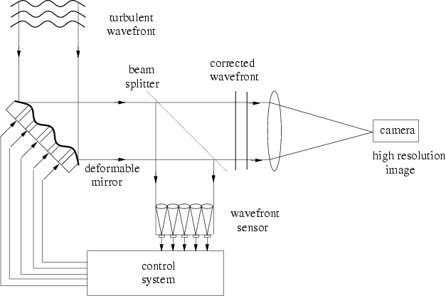 |
One of the main problem with adaptive optics is that the images are
never fully corrected. To understand that, we look at
Figure 1, showing the traditional lay-out of an AO
system: the turbulent wave-front is corrected by means of a deformable
mirror and the corrected wave-front is directed toward a science camera
to produce a high-resolution image. Because the atmospheric turbulence
is changing continuously, the shape of the deformable mirror that
corrects the wave-fronts must be updated continuously. To this effect, a
beam-splitter collects part of the corrected wave-front (either from
the object itself or from a nearby guide source) and sends it to a
wave-front sensor. The wave-front sensor measures the residual
aberrations in the corrected wave-front and a control computer determines
the commands to cancel these aberrations and applies them to the
deformable mirror. In order to keep up with the turbulence, an update
rate of typically 1 kHz is required. There are them several reasons why
the correction can not be perfect:
- The deformable mirror has a finite number of degrees of freedom
(actuators) and therefore is not able to perfectly reproduce the
turbulent wave-front;
- The wave-front sensing entails detecting photons from the guide
source in a very short time, typically a millisecond. Except when the
system can use a very bright source, the photon noise and detector noise
introduce errors in the measurements of the residual wave-front and
these errors propagate through the AO loop. Similarly, the spatial
sampling of the wave-front is never sufficient and the subsequent
aliasing errors further degrade the correction;
- The latency due to the integration / read-out of the wave-front
sensor and to the computing time of the control computer introduce a
time delay in the AO loop. Any evolution with a time scale smaller than
this delay will remain uncorrected;
- Finally, differential aberrations after the beam-splitter, between
the imaging path and the wave-front sensing path will show-up in the
final image unless they are properly calibrated.
In addition, off-axis acquisitions, i.e. when the AO guide source is not
the science object itself, are affected by anisoplanatism errors due to
the distribution of the turbulence at different altitudes. These errors
start to significantly impact the quality of the image when the angular
distance between the science source and the guide source is larger than
the so-called isoplanatic patch, typically 20-30 arcsec.
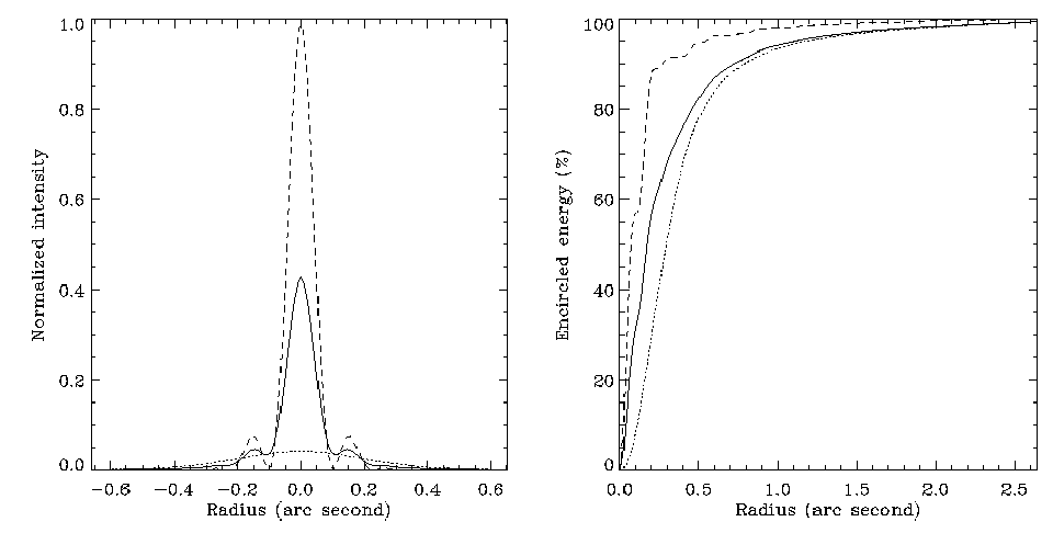
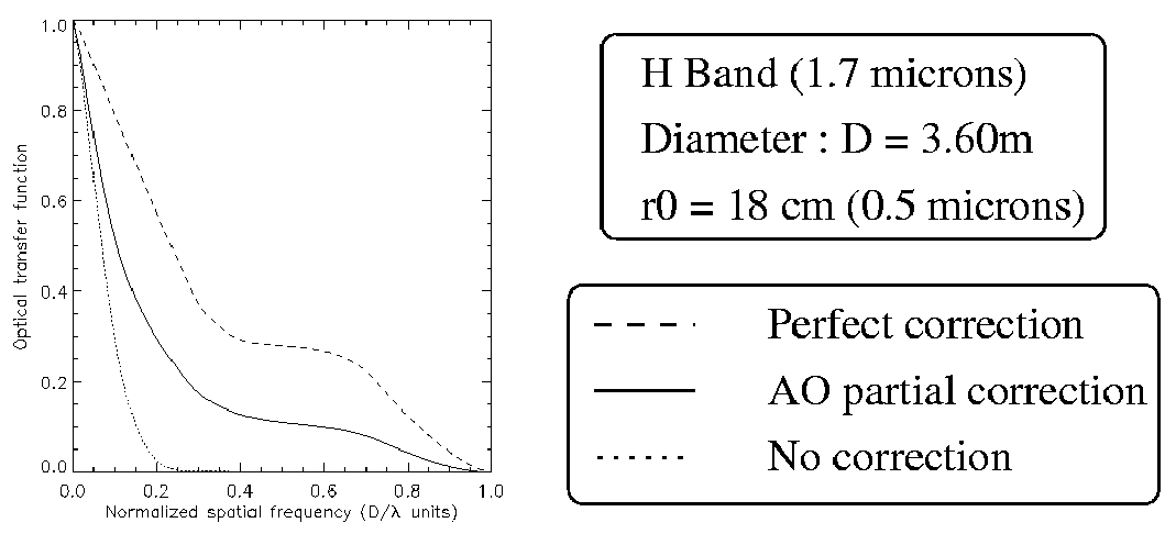
Thus, the AO correction is always partial. For most cases, this still allows
the image to achieve the maximal resolution of the telescope, that is
the image of a point source has a narrow central
core with a width given by the diffraction limit of the primary mirror.
However, because the
correction is partial, this central core contains only a fraction of the
total energy. The rest of the energy is scattered in an halo that extends
far away from the central core. The ratio of the energy contained in
the core to the total energy in the image is roughly what is referred to
as the Strehl ratio of the image: a Strehl ratio of 1 therefore
corresponds to a full correction. This effect is demonstrated in
Figure 2, where a fully corrected, AO partially corrected and
uncorrected images are plotted. The first plot shows a cut of the
three images scaled to the same energy. Note that the scaling factor
is chosen so that the vertical axis gives the Strehl ratio, with the
fully corrected image having a unity Strehl ratio. In this plot, we
can see that the AO corrected image has about the same full-width at
half maximum than the diffraction pattern. However, the central core
does not contain as much energy. The second plot of
Figure 2 shows the encircled energy of the three images,
that
is the fraction of energy as a function of the distance from the
center of the image. We can see that close to the center of the image,
the concentration of energy in the partially corrected image is about
as good as in the fully corrected image. However, far from the center,
in the wings of the image, the correction seems to be no longer effective and
the energy concentration in the partially corrected image and in the
uncorrected image is similar. The presence of this strong halo reduces
the contrast and smears the fine details of the image. This is clearly
shown in the third plot of Figure 2 that gives the
modulation transfer function (MTF) of the three images. We can see
that, contrary to the non-corrected image, the spatial content of the
partially corrected image is preserved up to the cut-off frequency of
the telescope. However, the amplitude of the MTF is reduced, compared
to the MTF of the fully corrected image.
Figure 2:
Comparison between an uncorrected image, an AO corrected image
and a diffraction limited image. Top left: image cut; Top right: encircled
energy plot; Lower left: modulation transfer function.
 |
 |
In the above, we have found that partially corrected images have
strong halo-like wings that extend many FWHM units from the center of
the image. Therefore, objects that are resolved by the AO system
contaminate each other through their halo. This effect prevents us from
detecting faint structures and from
extracting any quantitative information such as photometry from the
raw AO images. One of the most important step in the reduction of AO data
is therefore to reconcentrate the energy from the halo back to the
central core. This process is in fact deconvolution, but we note
that in the case of AO, the resolution is already granted by the
system. So it is important to insist that we do not seek to improve the
angular resolution of the
images, we just want to get rid of the halos. The successful
completion of this task leads to an increased contrast and therefore
a better detection of the faint structure in the image. Most
importantly, it allows astronomers to perform accurate quantitative
measurements on the image, such as photometry and astrometry.
If we neglect the spatial variation of the correction due to
anisoplanatism, all the information we need to remove the halo is
contained in the image of a point source or point spread function (PSF). In
an AO image, it is very rare that there is a point source isolated
enough so that the PSF can be obtained from its image. Then,
the AO PSF is very difficult to estimate: it has a very complex structure
(no analytical model) that changes with time as the observing
conditions (turbulence strength and speed) evolve. One possibility is
to give up on PSF estimation altogether and use blind deconvolution
schemes (Kundur et al. 1996) to extract both the underlying object and the
PSF only from the image. However, such methods are usually
artifact-prone and plagued with numerical instabilities. In astronomy,
they can be
applied only to very simple objects and/or require a very high
signal-to-noise ratio.
There are different ways to estimate the PSF related to any AO
image. It is important to understand these methods because of their
implication in the observing strategy at the telescope.
The default all-around method is to empirically obtain the PSF from
the image of a point source (star), taken before and/or after the
science acquisition. This PSF calibration operation must be planned in
advance by carefully selecting a calibration star that is close to the
object (at least same air-mass) and of same color and magnitude,
so that the AO correction is
the same for the object and
the calibration source. Observing with AO
very often leads to surprises, such as well-known guide stars turning out
to be close binaries or even more complex systems, making them unsuitable
to PSF calibration. It is therefore a very good idea to select at least
two calibration stars for each observation. One way to find
such calibration stars is to use on-line catalogs, such as the GSC or
USNO catalogs. Several interfaces to these catalogs exist, but the one
provided by the
Canadian Astronomy Data Centre
is very efficient and user friendly.
This empirical PSF determination method has several obvious
drawbacks though. The first one is the waste of observing time, with a
multi-million, very high resolution system, spending a significant portion
of time
observing an unresolved source. The second drawback is that since the
turbulence evolves in time, one is never quite sure that the calibrated
PSF will be accurate for the science acquisition. The only way around this
problem is to calibrate the PSF very frequently, which leads to even more
loss in observing time. The observer has also to contend with the
technical difficulty to make sure that the correction provided by the
AO system is the same for the science object and for the PSF star, that
is make sure that the WFS noise is the same, etc.
On CFHT, a much more efficient PSF determination method has been implemented
(Véran et al. 1997a).
It is an automatic method whereby the AO system determines its
own PSF by itself, using the real time data processed by the AO loop such as
the wave-front sensors measurements. This method runs in the AO real time
computer, in parallel with actual AO correction process. The advantage is
that the PSF reconstruction does not required any extra observing time and
that it uses data exactly synchronous to the acquisition. After each
acquisition, an extra file is produced, containing all the informations
required the reconstruct the PSF for this acquisition. The actual PSF
reconstruction is performed by the observer during the data reduction
stage. The reason why the PSF is not fully reconstructed on the fly by the
AO system is that the reconstruction still requires at least one image of a
point source, mostly to calibrate the non-common path aberrations.
There are, however, little constraints on when and how this point source should
be acquired. For instance, photometric calibration stars are a good choice.
More information on this can be found in reference Véran et al. (1997b).
This automatic PSF reconstruction method has been shown to give very
accurate PSF provided the guide source is magnitude 13.5 or brighter.
Unfortunately, it is so far only available on PUEO and while adapting it
to any other curvature system should be easy, this is not the case for
Shack-Hartmann systems because of intrinsic specificities. Work on this
problem is on-going in various AO teams.
This type of automatic PSF reconstruction method really seems to be the
way most AO system will operate in the future, that is when the difficulties
with the Shack-Hartmann systems will be solved. It is then critical that
any AO system be designed so that PSF files can be computed, saved and
archived routinely, in synchronization with each science acquisition.
Finally, one should also be aware of the two fundamental limitations
of this type of method:
- The PSF estimation is based on a statistical analysis of the AO data.
What is computed is therefore the long (infinite) exposure PSF. Even if
the estimation is perfect, this estimated PSF differs from the actual PSF
by the speckle noise. Speckle noise decreases as the exposure time increases.
For the estimated PSF to be useful, the exposure time should be typically
at least a few seconds;
- The PSF estimation is based on wave-front sensing data and is therefore
accurate in the direction of the AO guide source. Away from the guide source,
anisoplanatic effects will degrade the correction, and this degradation will
not be taken into account in the estimated PSF.
With a well calibrated / estimated PSF, one can try to deconvolve the
AO images. Again, this means trying to re-concentrate the flux in the halos
surrounding each point source back into the core associated to the source.
It is a well known fact that deconvolution is an ill-posed problem and
therefore prone to yield artifacts. There are two main forms of artifacts:
noise amplification and ringing. Because the images are always
recorded with an imperfect detector in a finite exposure time, low signal
regions are contaminated by noise, usually a combination of detector and
photon noise. The essence of deconvolution is to attempt to find an
underlying object ``consistent'' with the data, that is the object
convolved by the PSF should be ``consistent'' with the data. ``Consistent''
is of course the operative word. If no special care is taken the deconvolution
algorithm may try to fit the noise. Because the PSF is essentially a low
pass filter, small noisy bumps can only be fitted if large spikes are
introduced in the estimated object. This is how noise amplification occurs.
The second type of artifact, ringing, is not related to noise and can
appear even in noiseless data. Contrary to noise amplification which
affects the deconvolved image more or less uniformly, ringing appears in
the vicinity of sharp discontinuities in the object, such as point sources
or edge of planetary disks. Ringing manifests itself as a set of rings,
whose intensity decreases as one moves away from the discontinuity.
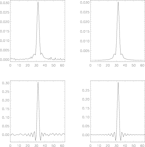
Ringing and noise amplification artifacts are illustrated by figure
3, where the image of a point source (typical AO PSF)
is deconvolved
by itself using a simple inverse filter. The important thing here is
to look at the vertical axis. Indeed, the deconvolution process results
in a much higher flux concentration in the central core. But artifacts are
evident: amplified noise + ringing in the noisy case (left) and ringing
only in the noiseless case (right). In both cases obviously, an extended
emission around the star would be destroyed by the artifacts.
Figure 3:
Illustration of the classical deconvolution artifacts. Top left:
PSF + noise; bottom left: PSF + noise deconvolved by PSF; top right:
PSF; bottom right: PSF deconvolved by PSF.
 |
There exists a range of general purpose deconvolution methods, available
within traditional astronomical processing softwares such as IRAF, MIDAS
and IDL. These methods apply to any kind of image, requires no or few
parameters setting and are therefore very easy to use. They come in
different names and flavors: the linear method of choice is the Wiener
filter (Andrew et al. 1977) and is well behaved in the sense that it is
not iterative and therefore there is no ambiguity in
stopping the algorithm. Non-linear methods such as Lucy Richardson
(Richardson 1972, Lucy 1974) and
Maximum Entropy (Narayan & Nityananda 1986)
are non-linear so they can enforce the positivity
of the estimated object, which is of great help to reduce the artifacts if
the background is indeed zero, that is there is no extended emission.
On the other hand, these algorithms are iterative and usually an ad-hoc
criterion must be use to decide when to stop the iterations.
While these general purpose methods are useful for a first look at the images,
they can usually be outperformed by methods where some strong constraints
on the object can be introduced. We explore those below.
Planets and planetary objects
These objects are usually extended bright object and can
be recorded with a very high SNR. For these objects, noise amplification
is not a worry, but ringing is, because the edge of the object is a very
sharp discontinuity in the image. Virtually all the general purpose
methods cited below would result in ringing effects on the surface of
the planet, preventing any attempt of photometric measurements for instance.
Recently, a specific method where such large discontinuities are explicitly
expected has been proposed and has already been used with success.
Stellar fields
Whether they are dense globular clusters or simple binary stars, stellar
fields have in common that we know a priori that they are a collection
of unresolved point sources with no extended emission, except maybe some
constant background. Then restoring the object as a pixel map is a poor
approach to the problem. Much better is to consider that the object
is a set of Dirac impulses whose positions (astrometry) and amplitudes
(photometry) are unknown. Well known methods to deal with this problem
include CLEAN and DAOPHOT. In some cases, these can be outperformed
by newer methods, such as AOPHOT (Véran et al. 1998) or the method
from reference Currie et al. (2000),
which are more specifically adapted to AO imaging.
Point sources super-imposed on an extended emission
These are the most difficult objects to deconvolve but they are also the
most common. The point sources are liable to introduce ringing whereas
the extended emission usually has low SNR and is very sensitive to noise
amplification. Specific methods to deal with this type of objects include
Lucy et al. (1994 - PLUCY method), Magain et al. (1998) and Hook et
al. (2000 - CPLUCY method). An other potentially powerful method but
with which we
do not have any first hand experience is the so-called ``Pixons'' method
(Pina & Puetter 1993, Puetter & Yahil 1998).
It may happen sometimes that the PSF can not be estimated with enough
accuracy. This is the case for example if the AO guide source is too faint or
if the acquisition is off-axis.
In that case, one might try to refine the PSF estimation
during the deconvolution itself. This process is referred to ``myopic
deconvolution'', because the initial estimate of the PSF is still
reasonable, as opposed to blind deconvolution, where no assumption on
the PSF is made. Recent work on blind deconvolution methods for AO includes
Christou et al. (1998) and Fusco et al. (1999).
When the observed field is larger than the isoplanatic patch, the PSF
significantly varies across and the deconvolution becomes very tricky.
This problem has only received little attention so far, probably because
the modest size of the current infrared detectors does not allow them
to cover a very large field, as the pixel size must be small enough to
sample adequately the AO corrected PSF. However, as the detectors get
bigger and
the AO correction is achieved at lower wavelength (the isoplanatic patch
decreases with the wavelength), this problem will become more critical.
To our knowledge, the only method that specifically addresses this problem
is the DAOPHOT algorithm for stellar fields, which take into account
a possible spread of the PSF in the field.
In this paper, we hope we have been able to convey that post-processing
of the data acquired with adaptive optics is absolutely crucial
to extract useful scientific informations from them. One of
the main difficulty is to obtain an accurate estimate of the AO PSF.
This requires a careful design of the AO system itself
and of the data handling system that supports it, as well as a careful
preparation and execution of the AO observations. With good quality
data and PSFs, accurate deconvolutions can be performed, but one should
watch carefully for artifacts such as noise amplification and ringing.
To avoid those, it is recommended to use, whenever possible, an object
specific deconvolution method, where strong a priori informations on the
underlying object are included, as opposed to general purpose methods.
References
Andrew, H., & Hunt, B. 1977, Digital Image Restoration, Prentice Hall
Christou, J. C., Marchis, F., Ageorges, N., Bonaccini, D., &
Rigaut, F. J. 1998, Proc. Spie, 3353, 984
Currie, D., et al. 2000, this volume, 381
Fusco, T., Véran, J.-P., Conan, J.-M., & Mugnier, L. M. 1999,
A&AS, 134, 193
Hook, R., et al. 2000, this volume, 521
Kundur, D., & Hatzinakos, D. 1996, IEEE Sig. Proc. Mag., 13, 43
Lucy, L. B. 1974, ApJ, 79, 745
Lucy, L. B. 1994, The Restoration of HST Images and Spectra II,
Hanish and White Eds., 79
Magain, P., Courbin, F., & Sohy, S. S., 1998, ApJ, 494, 472
Narayan, R., & Nityananda, R. 1986, ARA&A, 24, 127
Pina, R. K., & Puetter, R. C. 1993, PASP, 105, 630
Puetter, R. C., & Yahil, A. 1998, in ASP Conf. Ser., Vol. 172, Astronomical Data
Analysis Software and Systems VIII, ed. D. M. Mehringer, R. L. Plante, &
D. A. Roberts
(San Francisco: ASP), 307
Richardson, W. 1972, Journ. Opt. Soc. Am., 62, 55
Véran, J.-P., Rigaut, F., Maître, H., & Rouan, D. 1997, Journ. Opt. Soc. Am. A, 14, 3057
Véran, J.-P., Rigaut, F., Maître, H., & Rouan, D. 1997b, Proc. Spie, 3126, 81
Véran, J.-P., & Rigaut, F. 1998, Proc. Spie, Vol. 3353, 426
© Copyright 2000 Astronomical Society of the Pacific, 390 Ashton Avenue, San Francisco, California 94112, USA
Next: GBT Active Optics Systems and Techniques
Up: Adaptive and Active Optics
Previous: Adaptive and Active Optics
Table of Contents -
Subject Index -
Author Index -
PS reprint -
adass@cfht.hawaii.edu