The problem of doing accurate stellar photometry with calibrated charge-coupled device (CCD) data amounts to that of condensing the intensity values of hundreds, thousands, or even millions of picture elements (pixels) into a list containing the magnitude and position of each star on the CCD image.
If the stellar field is not crowded, the astronomer can measure the magnitude of each star by doing the digital equivalent of aperture photometry. Stellar photometry becomes much more difficult if one wishes to study crowded stellar fields. The basic assumptions underlying the simple techniques of CCD aperture photometry are frequently not valid in crowded stellar fields and more sophisticated methods like Point-Spread-Function (PSF) model fitting must be used in order to achieve accurate photometry.
The process of determining the apparent magnitude of a star can be surprisingly complex even with a technique as simple as CCD aperture photometry. We start by assuming that our CCD observations have already been flat-fielded and calibrated. The basic process of aperture stellar photometry is, in principle, quite simple:
There are many techniques available for the detection of astronomical objects in CCD observations (see, e.g., Fischer & Kochanski 1994, Secker 1995, and references therein). The following is a short introduction to some of the techniques that can be used to detect stars in CCD observations.
The signal of a noisy digital image can frequently be enhanced by
suppressing high spatial frequency noise in the image.
For modern CCD stellar observations, this generally means suppressing
photon and CCD readout noise.
This can frequently be accomplished by using small digital low-pass
filters like
The following listing, for example, is a FORTRAN implementation of a simple peak detector algorithm which identifies any pixel that is greater than any of its eight neighbors:
C
C A Simple Peak Detector Algorithm
C
C Copyleft (L) 1998 Kenneth J. Mighell (Kitt Peak National Observatory)
C
      SUBROUTINE PEAKER(IMAGE,NX,NY,PEAKMIN,PEAKMAX)
      INTEGER NX, NY, X, Y, XX, YY
      REAL    IMAGE(NX,NY), PEAKMIN, PEAKMAX, PIXEL, NEIGHBOR
      LOGICAL BINGO
      DO Y = 2,(NY-1)
      DO X = 2,(NX-1)
      PIXEL = IMAGE(X,Y)
      IF ((PIXEL.GE.PEAKMIN).AND.(PIXEL.LT.PEAKMAX)) THEN
        BINGO = .TRUE.
        DO YY = (Y-1),(Y+1)
        DO XX = (X-1),(X+1)
          IF (BINGO) THEN
            NEIGHBOR = IMAGE(XX,YY)
            IF (NEIGHBOR.GT.PIXEL) THEN
              BINGO = .FALSE.
            ELSE IF (NEIGHBOR.EQ.PIXEL) THEN
              IF ((XX.NE.X).OR.(YY.NE.Y)) THEN
                IF (((XX.LE.X).AND.(YY.LE.Y))
     &             .OR.((XX.GT.X).AND.(YY.LT.Y))) BINGO = .FALSE.
              ENDIF
            ENDIF
          ENDIF
        ENDDO
        ENDDO
        IF (BINGO) WRITE (*,*)
     & 'Found a peak at position (',X,',',Y,') with a value of',PIXEL
      ENDIF
      ENDDO
      ENDDO
      RETURN
      END
C23456
This algorithm works particularly well with
CCD stellar observations that have had the background sky
removed (e.g., LPD-filtered images).
Many CCD aperture photometry programs require the user to give the position of the star on the CCD frame. Most of these programs offer a choice of centering algorithms to determine the center of a star when provided with only a rough estimate. The review article of Stone (1989) compares the performance of five different digital centering algorithms under a wide range of atmospheric seeing and background-level conditions. It may be useful to create your own centroid algorithm based upon the special requirements of your particular analysis problem. The following listing, for example, is a FORTRAN implementation of a centroid algorithm which produces robust estimates without requiring an estimate of the the nearby ``sky'' background:
C
C A Simple Centroid Algorithm
C
C A modification of the Modified Moment Method (Stone 1989,AJ,97,1227)
C that works well with small apertures.
C
C Copyleft (L) 1998 Kenneth J. Mighell (Kitt Peak National Observatory)
C
      SUBROUTINE CENTROID(X,Z,NN,N,X_IN,X_OUT)
      INTEGER          N, NN ! <-- assumes that 1 <= N <= NN
      REAL             X(NN), Z(NN), X_IN, X_OUT, BIG
      DOUBLE PRECISION DELTA, SUM1, SUM2, DIFF, XX
      DOUBLE PRECISION INTENSITY, POSITION, MINIMUM
      INTEGER          I, J , NITERATIONS
      PARAMETER        (BIG=1E30,NITERATIONS=10)
      MINIMUM = BIG
      DO I = 1,N
        INTENSITY = Z(I) ! <-- Z(I) is the intensity at the position X(I)
        MINIMUM = MIN(INTENSITY,MINIMUM)
      ENDDO
      XX = X_IN
      DELTA = 0D0
      DO J = 1,NITERATIONS
        XX = XX + DELTA
        SUM1 = 0D0
        SUM2 = 0D0
        DO I = 1,N
          POSITION = X(I)
          INTENSITY = Z(I)
          DIFF = MAX((INTENSITY-MINIMUM),0D0)
          SUM1 = SUM1 + (POSITION-XX)*DIFF
          SUM2 = SUM2 + DIFF
        ENDDO
        DELTA = SUM1/SUM2
      ENDDO
      X_OUT = XX
      RETURN
      END
C23456
This algorithm is a simplified version of the one used by my
CCDCAP aperture stellar photometry
package.
If precise absolute or relatives positions from CCD observations
are required, then one should investigate the extensive literature
dedicated to CCD astrometry.
The background (``sky'') flux associated with a star is generally determined
by analyzing the distribution of intensities of nearby background pixels.
In the case of circular aperture photometry,
the background flux is typically determined by analyzing the pixels
in an annulus beyond the stellar aperture.
The inner radius of the sky annulus
is typically several FWHM1distant from the center of the aperture
in order to avoid the inclusion of contaminating light from the star itself.
The width of the annulus is typically large enough
so that the annulus contains between ![]() 50 and
a few hundred pixels.
50 and
a few hundred pixels.
Many aperture photometry programs allow the user to set the
background flux to be the modal value
of the background intensity distribution.
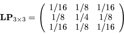
The mode of the background distribution is frequently estimated
by using the following useful approximation,
Many algorithms are available and most aperture photometry programs offer the user a choice of several methods to determine the background flux. For example, the popular APPHOT aperture photometry IRAF package offers the user the choice of 11 different ways the background can be estimated (Davis 1987). As always when using analysis software, the astronomer is strongly advised to carefully read the user documentation in order to understand which methodology will produce the best results for a given CCD observation or application.
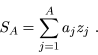
The fundamental task of a CCD aperture photometry program
is to accurately measure all the electrons,
SA,
that fall within an aperture placed on a CCD image.
Unless the background flux, B, is exactly zero
electrons per pixel, one can never directly measure
the number of electrons, ![]() , from a star within the
aperture.
One measures, instead, the quantity
, from a star within the
aperture.
One measures, instead, the quantity
![]() ,
where
,
where ![]() is the aperture of the aperture (in pixels).
The instrumental magnitude of an
aperture measurement of a CCD observation of a star
can thus be defined as
is the aperture of the aperture (in pixels).
The instrumental magnitude of an
aperture measurement of a CCD observation of a star
can thus be defined as
It is clearly important to determine the observable quantities
SA, B, and ![]() as accurately as possible.
Let us consider the aperture area,
as accurately as possible.
Let us consider the aperture area, ![]() , first.
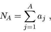
If aj is the area of the jth aperture pixel, then
the total area of the aperture,
, first.
If aj is the area of the jth aperture pixel, then
the total area of the aperture, ![]() , is simply
, is simply
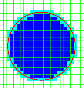 |
Let us now consider the sum of all electrons within the aperture (SA).
If zj is the intensity (in electrons) of the jth aperture pixel,
then one simple approximation of SA is
One way of reducing this systematic measurement error is to
split each pixel into subpixels by using a bilinear pixel
interpolation algorithm. One such algorithm is to use the
two-dimensional analog of the sinc function: ![]() .
This function, like many others, has the unfortunate effect
of degrading the original image by spreading photons (electrons)
beyond the original pixel.
I created created the
QUADPX
bilinear pixel interpolation
algorithm which splits
a pixel into 4 subpixels whose sum is always equal to that
of the original pixel (Appendix B of Mighell & Rich 1995).
Numerical experiments have shown that using the QUADPX algorithm
can reduce the systematic measurement error of
critically-sampled Gaussians
by a factor of
.
This function, like many others, has the unfortunate effect
of degrading the original image by spreading photons (electrons)
beyond the original pixel.
I created created the
QUADPX
bilinear pixel interpolation
algorithm which splits
a pixel into 4 subpixels whose sum is always equal to that
of the original pixel (Appendix B of Mighell & Rich 1995).
Numerical experiments have shown that using the QUADPX algorithm
can reduce the systematic measurement error of
critically-sampled Gaussians
by a factor of ![]() 6.
For example, the photometric error of an aperture radius
of 2.0 pixels went from 0.068 mag using Equation (1) to
0.011 mag with the CCDCAP package which implements the QUADPX
algorithm.
6.
For example, the photometric error of an aperture radius
of 2.0 pixels went from 0.068 mag using Equation (1) to
0.011 mag with the CCDCAP package which implements the QUADPX
algorithm.
The best (smallest) stellar photometric errors (i.e., the largest signal-to-noise ratios) are generally obtained with relatively small apertures (see, e.g., Fig. 6 of Howell 1989). Analysis of theoretical CCD signal-to-noise-ratio equations (see, e.g., Newberry 1991, Howell 1992, Merline & Howell 1995, Howell et al. 1996, and references therein) shows that large apertures can have large photometric errors when the the total number of stellar photons in the aperture becomes comparable with the total number of background photons in the aperture. Furthermore, a measurement error for the background flux as small as just 1 electron per pixel can by itself produce large photometric uncertainties at large aperture radii. Small apertures, however, can be too small when they allow such a small fraction of the star light to be found within the aperture that the photometric error becomes dominated by small-number (a.k.a. counting or Poisson) statistics because little or no signal has been measured.
A Gaussian is a good model for
the Point Spread Function of a ground-based CCD observation
since the central core of a ground-based stellar profile is approximately
Gaussian (King 1971).
One can easily show that the optimum signal-to-noise ratio
for a Gaussian PSF is obtained for a circular aperture radius of
![]() 1.6
1.6![]() (i.e.,
(i.e.,
![]() FWHM)
which contains about 72% of the encircled-energy.
Pritchet & Kline (1981) note that
the signal-to-noise ratio is fairly insensitive to radius near the
``optimal'' radius value
FWHM)
which contains about 72% of the encircled-energy.
Pritchet & Kline (1981) note that
the signal-to-noise ratio is fairly insensitive to radius near the
``optimal'' radius value ![]() 1.6
1.6![]() for a Gaussian PSF;
deviations from the optimal radius by as much as
for a Gaussian PSF;
deviations from the optimal radius by as much as
![]() 50% generally make little difference.
Since centering errors will be more critical for smaller apertures
than for larger apertures, it is only prudent to err on the larger side by
using apertures with radii which are larger than
50% generally make little difference.
Since centering errors will be more critical for smaller apertures
than for larger apertures, it is only prudent to err on the larger side by
using apertures with radii which are larger than
![]() 0.68
0.68![]() FWHM.
FWHM.
An aperture radius of ![]() FWHM makes an excellent practical
compromise between concerns about systematic centering errors and
diminishing signal-to-noise ratios typically obtained
with larger aperture radii.
By analyzing the CCD signal-to-noise ratio equations, one can show that
brighter stars will have larger optimal aperture sizes than do
fainter stars.
If one must use only one aperture size, then it is
clearly advantageous to chose a global aperture size which produces
the smallest photometric errors for the faintest stars
(i.e., use
FWHM makes an excellent practical
compromise between concerns about systematic centering errors and
diminishing signal-to-noise ratios typically obtained
with larger aperture radii.
By analyzing the CCD signal-to-noise ratio equations, one can show that
brighter stars will have larger optimal aperture sizes than do
fainter stars.
If one must use only one aperture size, then it is
clearly advantageous to chose a global aperture size which produces
the smallest photometric errors for the faintest stars
(i.e., use ![]() FWHM).
FWHM).
Small apertures frequently do not contain all the flux from a star. The amount of the missing star light can found by determining the appropriate aperture correction by measuring nearby bright isolated stars. Howell (1989) and Stetson (1990), among others, describe the process how aperture corrections can be accurately determined using the aperture growth-curve method.
Consider a ground-based CCD observation of two stars whose stellar images overlap. Assuming we already know the Point Spread Function of the observation, a simple model of the observation will have seven parameters: peak intensities (I1,I2), positions (X1,Y1,X2,Y2), and the background sky level B which is assumed to be the same for both component images. One finds that the parameters are not independent for overlapping stars with the presence of photon and readout noise. The conservation of photon flux will require that if I1 increases then I2 must decrease and vice versa for a given value of B. The most accurate photometry possible is obtained when these dependent parameters are fitted simultaneously. Any reasonable model of two overlapping stellar images will be a non-linear function when the positions and peak intensities are to be determined simultaneously. The technique of non-linear least-squares fitting was developed to provide for the simultaneous determination of dependent or independent parameters of non-linear model functions.
Assume that we
have a calibrated CCD observation with N pixels
and that zi
is the intensity in electrons (e-)
of the ith pixel at (xi,yi) with an error
of ![]() . Let
. Let
![]() a1,
a1,![]() aM)
be a model of the intensity values that has two coordinates
(x,y) and M parameters.
For notational convenience, let the vector
ri represent the coordinates (xi,yi)
and the vector a represent all the parameters
[i.e.,
aM)
be a model of the intensity values that has two coordinates
(x,y) and M parameters.
For notational convenience, let the vector
ri represent the coordinates (xi,yi)
and the vector a represent all the parameters
[i.e.,
![]() ].
Thus the model of intensities will normally be written as
].
Thus the model of intensities will normally be written as
![]() .
.
The measure of the goodness of fit between the
data and the model, called chi-square,
is defined as
![\begin{displaymath}
\mbox{$\chi^2(\mbox{\boldmath$a$})$}\equiv \sum_{i=1}^{N}
\f...
...em {model}}(\mbox{\boldmath$r$}_i;\mbox{\boldmath$a$})]^2\ \ .
\end{displaymath}](img35.gif)
For some small correction parameter vector
![]() we can approximate
we can approximate
![]() by its Taylor series
expansion:
by its Taylor series
expansion:
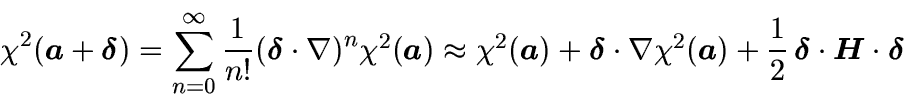
This method will find the absolute minimum of
![]() if the original
guess
if the original
guess
![]() is near
is near
![]() .
Unfortunately, the original guess of the parameter vector
.
Unfortunately, the original guess of the parameter vector
![]() may not always be very good. For production stellar photometry software
it is important that the search
for the absolute minimum of
may not always be very good. For production stellar photometry software
it is important that the search
for the absolute minimum of ![]() be both robust
and efficient.
be both robust
and efficient.
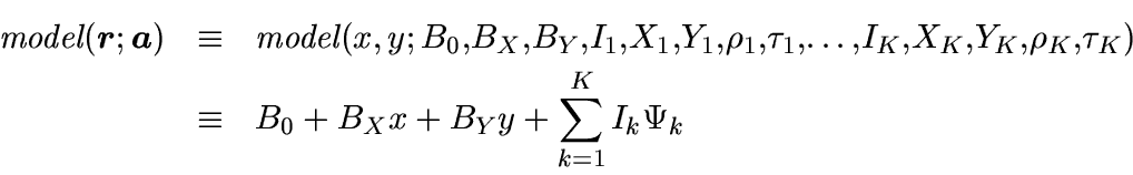
One can frequently create a realistic intensity model of a ground-based CCD
observation of a total of K stars on a non-flat background with
a combination of Moffat (1969) functions on a tilted plane:
![\begin{displaymath}
\mbox{$\gamma_k^{-\tau_k}$}
\equiv
\!\!\frac{1}{\eta^2}
\sum...
...i+\eta^{-1}j]-\!Y_k)^2
}{\rho_k^2}
\right\}
\right]^{-\tau_k}
\end{displaymath}](img59.gif)
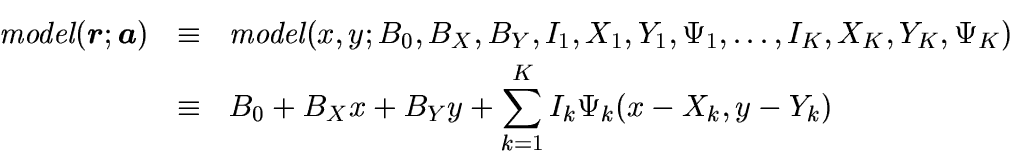
One can create a realistic intensity model of a
Hubble Space Telescope ( HST)
CCD observation of K stars on a non-flat background with
a combination of
digital Point Spread Functions
on a tilted plane:
![\begin{minipage}[h]{\textwidth} %5.25truein\}
\vspace*{-105truemm}
\hspace*{-5...
...textwidth}
{\bf {\hskip 26truemm}{WFPC2}{\hskip 49truemm}{WF/PC}}
\end{minipage}](img66.gif) |
Traditional PSF-fitting CCD photometric reduction packages like
DAOPHOT
(Stetson 1987) use analytical functions to represent the Point Spread Function.
All the major partial derivative
computations are computed on the analytical model of the PSF.
Any deviations of the real-world PSF from the analytical PSF
are then generally stored in a residual matrix which is only used
to determine the ![]() goodness-of-fit.
goodness-of-fit.
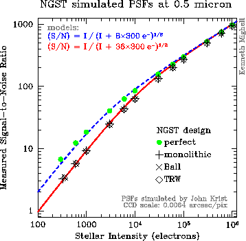
I have recently demonstrated the feasibility of doing accurate CCD stellar photometry with digital Point Spread Functions. I have developed a new digital PSF-fitting algorithm which does not require a residual matrix because all partial derivative computations are done on the digital PSF itself using standard numerical differentiation techniques. This algorithm has already passed the proof-of-principle stage with the successful reduction of simulated Next Generation Space Telescope (NGST) CCD stellar observations (see Fig. 3.).
I investigated the performance of CCD stellar photometry with a 1.5-micron diffraction-limited 8-m Next Generation Space Telescope. These simulations used artificial Point Spread Functions for three different 8-m NGST design concepts which were kindly provided by John Krist. Assuming that the 8-m NGST primary mirror has 1/13 wave RMS errors at 1.5 micron, I determined that 90% of the light from a star falls within an aperture radius of 0.1 arcsec -- the size of one WF pixel of the Hubble Space Telescope WFPC2 instrument. The three NGST design concepts have nearly identical V-band encircled-energy functions; the degradation caused by the differences between the three NGST design concepts is quite negligible when state-of-the-art digital-PSF photometric reduction software is used to analyze uncrowded stellar fields.
 |
Arfken, G. 1970, Mathematical Methods for Physicists (2nd ed.), (New York: Academic Press)
Da Costa, G. S. 1992, in ASP Conf. Ser., Vol. 23, Astronomical CCD Observing and Reduction Techniques, ed. S. B. Howell, (San Francisco: ASP), 90
Davis, L. 1987, ``Specifications for the Aperture Photometry Package'', National Optical Astronomy Observatories, ftp://iraf.noao.edu/iraf/docs/apspec.ps.Z
Fischer, P. & Kochanski, G. P. 1994, AJ, 107, 802
Haldane, J. B. S. 1943, Biometrika, 32, 294
Howell, S. B. 1989, PASP, 101, 616
![]() , 1992, in ASP Conf. Ser., Vol. 23,
Astronomical CCD Observing and Reduction Techniques,
ed. S. B. Howell, (San Francisco: ASP), 105
, 1992, in ASP Conf. Ser., Vol. 23,
Astronomical CCD Observing and Reduction Techniques,
ed. S. B. Howell, (San Francisco: ASP), 105
Howell, S. B., Koehn, B., Bowell, E., & Hoffman, M. 1996, AJ, 112, 1302
Irwin, M. J. 1985, MNRAS, 214, 575
Kendall, M. G. & Stuart A. 1958, The Advanced Theory of Statistics, Vol. I, (London: Charles Griffin & Co.) pp. 39 and 179
King, I. R. 1971, PASP, 83, 199
Krist, J. 1993, in ASP Conf. Ser., Vol. 52, Astronomical Data Analysis Software and Systems II, ed. R. J. Hanisch, R. J. V. Brissenden, & J. Barnes (San Francisco: ASP), 530
![]() , 1994, Tiny Tim User's Manual (Ver. 4.0)
, 1994, Tiny Tim User's Manual (Ver. 4.0)
Krist, J. & Hook, R. 1997, Tiny Tim User's Guide (Ver. 4.4)
Levenberg, K. 1944, Quart. of Appl. Math., 2, 164
Malin, D. 1977, AAS Photo-Bull., No. 16, 10
![]() , 1981, J. Phot. Sci., 29(5), 199
, 1981, J. Phot. Sci., 29(5), 199
Marquardt, D. 1963, J. SIAM, 11, 431
Merline, W. J. & Howell, S. B. 1995, Exp. Astron., 6, 163
Mighell, K. J. 1989, MNRAS, 238, 807
![]() , 1990, A&AS, 82, 1
, 1990, A&AS, 82, 1
Mighell, K. J. & Rich, R. M. 1995, AJ, 110, 1649
Moffat, A. F. J. 1969, A&A, 3, 455
Newberry, M. V. 1991, PASP, 103, 122
![]() , 1992, in ASP Conf. Ser., Vol. 25, Astronomical Data Analysis
Software and Systems I, ed. D. M. Worrall, C. Biemesderfer, &
J. Barnes (San Francisco: ASP), 307
, 1992, in ASP Conf. Ser., Vol. 25, Astronomical Data Analysis
Software and Systems I, ed. D. M. Worrall, C. Biemesderfer, &
J. Barnes (San Francisco: ASP), 307
Pearson, K. 1895, Phil. Trans., 186, 343
Press, W. H., Flannery, B. P., Teukolsky, S. A., & Vetterling, W. T. 1986, Numerical Recipes, (Cambridge: Cambridge Univ. Press)
Pritchet, C. & Kline, M. I. 1981, AJ, 86, 1859
Secker, J. 1995, PASP, 107, 496
Stetson, P. B. 1987, PASP, 99, 191
![]() , 1990, PASP, 102, 932
, 1990, PASP, 102, 932
Stone, R. C. 1989, AJ, 97, 1227
Wells, D.C. 1979, in SPIE Proc., Vol. 172, Instrumentation in Astronomy III, ed. D. L. Crawford, (Bellingham: SPIE), 418
![\begin{displaymath}
\mbox{$\Psi$}_k
\equiv
\int_{x-0.5}^{x+0.5}
\int_{y-0.5}^{y+...
...\rho_k^2}
\right\}
\right]^{-\tau_k}
\mbox{d}y
\
\mbox{d}x
~.
\end{displaymath}](img52.gif)