I. C. Busko
Astrophysics Division,
National Space Research Institute, CP 515, CEP 12201-970,
S. J. dos Campos, SP, Brazil
The image formation process introduces uncertainties in pixel values, due to both deterministic (Point Response Function, PRF) and random (noise) effects. The traditional approach to this problem involves some sort of inversion technique, and these are usually unable to use optimally all of the information available both a priori and in the data. An alternative approach is to adopt a data modeling perspective of the imaging problem. The work reported here aims at developing Bayesian-inference signal modeling methods based on sampling techniques. These methods are able to provide optimal estimators for pixel values, but, more importantly, can also provide consistently their error bars, and confidence levels for detected structures in the image. Hypothesis testing capabilities can also be built-in in these methods, as well as the capability of handling complicated, non-analytic imaging models.
The goal of Bayesian inference in imaging problems is to compute the posterior probability density given by Bayes' rule

where
 is the data vector (observation),
 is the parameter vector to fit, and
 is the hypothesis space containing the model being fitted.
MAP (Maximum A Posteriori) estimation is the simplest Bayesian inference
operation; it corresponds to finding the posterior's maximum (mode). It is
relatively easy to perform since there is no need to compute the normalization
term  .
Several MAP methods exist, adapted to a variety of problems, usually
seeking the fastest way to the solution through the use of efficient
maximization algorithms.
If one wants more information on the posterior besides its mode,
sampling methods can be of help (Gelfand & Smith 1990), since they
offer a very general way of handling intractable probability densities.
Stochastic Relaxation (SR) is such a method, with foundations in
statistical physics.
It was devised to study equilibrium properties of large systems of identical
``particles''. When combined with an ``annealing schedule,'' SR can be used
as a maximization tool as well (Geman & Geman 1984;
Kirkpatrick et al. 1983).
It is robust (does not get stuck in secondary maxima), intrinsically parallel,
and very easy to code, in the sense that the algorithm does not depend on
the details of the imaging problem. Thus, it can easily take into account
such complicated imaging situations as signal-dependent noise,
variable/disjoint PRFs, and non-analytic prior densities
 . Thus, it is an excellent testbed for experimenting
with such imaging situations.
In this work an IRAF task that implements SR was created and is being tested with both artificial and actual ROSAT HRI data. The task can be used either as a MAP searcher or as a Gibbs sampler for the posterior density (Geman & Geman 1984), and includes both Maximum Likelihood (ML) and Maximum Entropy (ME) prior densities. An on-axis PRF was computed by task rosprf in the xray package and used in all experiments.
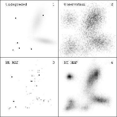
Figure ![]() depicts MAP solutions obtained by the SR algorithm with
both ML and ME priors, using as input a simulated ROSAT HRI observation.
The Richardson-Lucy (R-L) algorithm is used here as comparison, since it
is the Expectation Maximization implementation of ML for Poisson data.
depicts MAP solutions obtained by the SR algorithm with
both ML and ME priors, using as input a simulated ROSAT HRI observation.
The Richardson-Lucy (R-L) algorithm is used here as comparison, since it
is the Expectation Maximization implementation of ML for Poisson data.

Figure:
Panel 1: artificial sky field.
Panel 2: 10,000 photon simulated ROSAT HRI observation.
Panel 3: ML MAP estimator. The same result is obtained by either SR
or R-L.
Panel 4: ME MAP estimator, obtained by SR.
Original PostScript figure (533 kB)
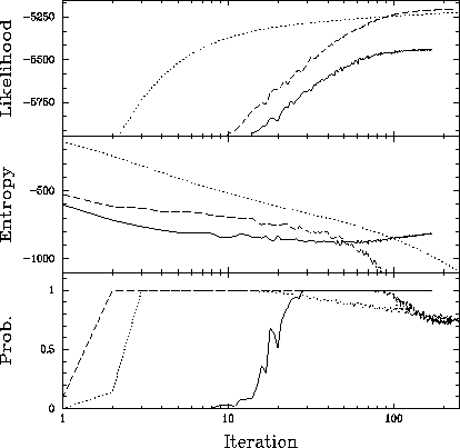
Figure ![]() depicts values assumed by the likelihood
depicts values assumed by the likelihood
 and prior
  densities along the iteration sequence for each algorithm.
The likelihood can be expressed in a zero-to-one probability scale by the
bootstrap sampling technique of Bi & Boerner (1994). In this way, it is a
measure of how well a given estimator ``fits the data.''
Notice how the likelihood increases monotonically with iteration number,
while probability for both ML and R-L reaches a maximum and decreases
afterwards. This behavior, which is also seen with actual ROSAT data,
was used to define a ``best'' estimator, which is the last one
along the iteration sequence for which the likelihood, as expressed in a
probability scale, is
  . In other words, the best estimator is the
most restored one which still fits the data with high probability.
In this experiment, the best R-L estimator
appears at iteration
  , best ML at iteration
  , and best ME
at convergence. This ME estimator is depicted in Panel 4 of Figure
 ![]() .
Figure
.
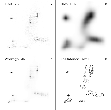
Figure ![]() depicts the best ML and R-L estimators.
depicts the best ML and R-L estimators.

Figure:
Likelihood (log), entropy and probability for ROSAT HRI simulated data, along
the iteration sequence of each algorithm.
Solid: SR with entropy prior.
Dashed: SR with Maximum Likelihood prior.
Dotted: Richardson-Lucy.
Original PostScript figure (48 kB)
When operated as a Gibbs sampler, SR output can be used along with the
ergodicity theorem of Geman & Geman (1984) to compute moments of
the posterior density. Figure ![]() depicts the first moment
for the ML prior. This is the posterior mean, which should be
compared with its mode in Panel 3 of Figure
depicts the first moment
for the ML prior. This is the posterior mean, which should be
compared with its mode in Panel 3 of Figure ![]() .
Panel 8 in Figure
.
Panel 8 in Figure ![]() depicts iso-confidence level contours
for the same prior. These were derived from both the first and second
moments of the posterior. They show that the extended structures detected
on the estimator are backed up by the data at the 1--2
depicts iso-confidence level contours
for the same prior. These were derived from both the first and second
moments of the posterior. They show that the extended structures detected
on the estimator are backed up by the data at the 1--2  level.
Stars are backed up by the data at the 3
  level and above.

Figure:
Panel 5: ``Best'' ML estimator obtained by SR.
Panel 6: Best R-L estimator.
Panel 7: Averaged Gibbs sampler output (150 samples) with ML prior.
Panel 8: Iso-confidence curves for Panel 7 estimator, ranging from
1 to 7  in steps of 1.
Original PostScript figure (533 kB)
Two main areas of future work are envisaged. The first is the inclusion of new prior types, such as Maximum Sparsity (Jeffs & Elsmore 1991) and Markov Random Field, and adaptation of the likelihood computation to specific problems (e.g., coded mask). The second is the implementation of a different sampling scheme, that would automatically and explicitly take care of the posterior normalization.
Gelfand, A. E., & Smith, A. F. M. 1990, J. Amer. Statist. Assoc., 85, 398
Geman, S., & Geman, D. 1984, IEEE Transactions on Pattern Analysis and Machine Intelligence, PAMI-6, 721
Jeffs, B. D., & Elsmore, D. 1991, International Conference on Acoustics, Speech and Signal Processing, ICASSP91-4, 2937
Kirkpatrick, S., Gelatt, C. D. Jr., & Vecchi, M. P. 1983, Science, 220, 671