The data from individual observations will be processed through a set of pipelines specific to the particular data collection mode, and an infrastructure has been implemented to enable the processing and quality assessment in a lights-out fashion (Moshir 2001). Typically for a given instrument, calibration data are first processed through a set of calibration pipelines and then the resulting calibration terms are employed during the reduction and calibration of regular science data products. A paper at this conference discusses the spectroscopic mode pipelines (Fang et al. 2003). The SIRTF Science Center (SSC) is committed to providing the user community the most up-to-date calibrated data products. As part of this commitment it is also planned to provide the users with estimates of product uncertainties that are traceable, reasonable, and at the same time informative.
In Section 2 we will first discuss some of the motivating concepts for this undertaking, and in Section 3 we will discuss the statistics and practical aspects of approaching the problem. Section 4 is devoted to a discussion of examples and complications. In Section 5 we discuss the issue of uncertainty propagation when calibration data are interpolated.
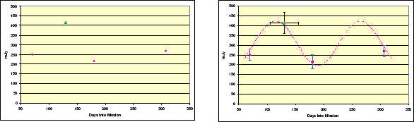
In many undertakings it is customary (due to diverse circumstances such as lack of resources, compressed schedules, etc.) to quote reasonable uncertainties--at times using somewhat ad-hoc methods. In our discussion, besides the requirement of reasonableness we wish to emphasize the adjective informative. It signifies that it is possible to make statistically significant statements regarding the quality of the data. An example of when correct and informative uncertainties provide significant aid in scientific utilization of the data can be seen in Figure 1. In the left panel the flux densities for a source quoted in the IRAS Faint Source Survey (Moshir et al. 1992) and IRAS pointed observations are shown. Without the ``error bars'' it would not be possible to conclude much about the detections, or even whether the data are trustable at all. However, with the uncertainties shown, it is possible to consider and evaluate several hypotheses to explain the disagreement between the two datasets. Here the hypothesis of a variable source appears to fit the data well (right panel). Later follow up of the source revealed that the object was in fact a variable star.
 |
In passing we note some areas where uncertainty analysis has been proven to be of significant utility:
In order to proceed with the program of uncertainty estimation and propagation, a few preliminaries need to be considered:
In many cases in the discussion of uncertainties there is an unspoken
assumption that prevails, namely that of normality. There are
many reasons for this. For example, Gaussian distributions are part of
every science curriculum. They are easy to manipulate and lead to rigorous justification
for least squares fit, ![]() minimization, and goodness of fit tests. The second
moments can be tied to confidence levels (1-
minimization, and goodness of fit tests. The second
moments can be tied to confidence levels (1-![]() and 68% probability
becoming interchangeable). And finally, under reasonable ( but not all)
conditions, many scenarios lead to Normal distributions.
and 68% probability
becoming interchangeable). And finally, under reasonable ( but not all)
conditions, many scenarios lead to Normal distributions.
It needs to be kept in mind that the assumptions of normality should not cloud
practical situations (where the statement ``let
![]() '' does
not clearly apply!) There are cases when uncertainties can not be treated
as Gaussian because data are a mixture of different distributions, for example
there are radiation hits, transients in the field of view, etc. There are
also cases where the instrumental noise does not follow a Gaussian model. And
an important often encountered situation is that mathematical operations on
Gaussian data can easily turn them into non-Gaussian constructs.
'' does
not clearly apply!) There are cases when uncertainties can not be treated
as Gaussian because data are a mixture of different distributions, for example
there are radiation hits, transients in the field of view, etc. There are
also cases where the instrumental noise does not follow a Gaussian model. And
an important often encountered situation is that mathematical operations on
Gaussian data can easily turn them into non-Gaussian constructs.
Despite all of the previous points and potential complications, one still
needs to estimate ![]() s that are reasonable and informative so they can
be used to signify confidence bands. These complications only make the subject
more interesting and reveal some new approaches in the field of practical
applications of statistics.
s that are reasonable and informative so they can
be used to signify confidence bands. These complications only make the subject
more interesting and reveal some new approaches in the field of practical
applications of statistics.
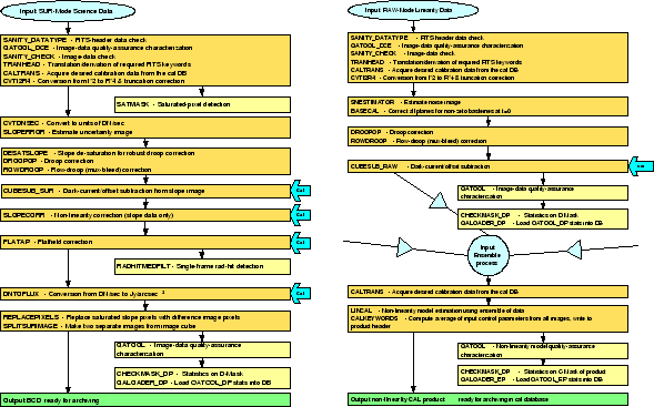
As an illustration of the scenarios we encounter, two pipelines, one for science and the other for calibration are shown in Figure 2. The science pipeline consists of a series of well defined arithmetical operations for which the rules of mathematical statistics provide the means of propagating the uncertainties. The science pipeline also applies calibration terms to the products using well defined mathematical operations; these steps are shown with a thick arrow. In these stages one must be aware of epoch differences between when the calibration measurements are performed and when the science data are collected. This leads to the issues of uncertainty propagation with sparse calibration terms, a subject that will be discussed in section 5. Similar considerations apply to the calibration pipeline shown in the right hand side panel of Figure 2.
 |
With the advent of sophisticated (and expensive!) instrumentation,
they are also becoming generally well characterizable. The noise model is
usually known to a reasonable extent. The model is generally verified in
lab tests, for example
through repeatability experiments. For a measured DN value one can write a
formula for the uncertainty that depends on the measured DN and a few other
characterized parameters (independent of DN value). For example via a simple
formula such as
![]() , where
, where ![]() is in
electrons,
is in
electrons, ![]() is the gain (in e-/DN) and
is the gain (in e-/DN) and ![]() is the ``read noise''
expressed in electrons; thus one may assign an
a priori uncertainty to each measured value. For a given
measurement
is the ``read noise''
expressed in electrons; thus one may assign an
a priori uncertainty to each measured value. For a given
measurement
![]() (
(
![]() ) it becomes possible to propagate
the uncertainties as the measurement progresses through pipelines. Now suppose
that the instrument's gain is not known at a given instance
(the physics of the detector would lead to a variable gain, for example
the transients in a Ge:Ga array). As a case study we consider the scenario
where it is only known that the gain is varying somewhere in the range of
3 to 8 e-/DN.
) it becomes possible to propagate
the uncertainties as the measurement progresses through pipelines. Now suppose
that the instrument's gain is not known at a given instance
(the physics of the detector would lead to a variable gain, for example
the transients in a Ge:Ga array). As a case study we consider the scenario
where it is only known that the gain is varying somewhere in the range of
3 to 8 e-/DN.
We desire the uncertainty distribution appropriate for photon noise (following
the common model of Poisson statistics) with
a gain that is variable or unknown. Photo-electron number is DN multiplied
by the gain ![]() . The gain is normally treated as a constant, but here the
problem is defined such that our lack of
knowledge of the gain (except that it is somewhere between 3 and 8!)
leads us to treat the gain as a random variable with a uniform distribution.
For example, a DN value of 1 may
imply anything from 3 to 8 photo-electrons with equal probability (again we
emphasize that the instrument is not acting randomly, it is
our state of knowledge that is incomplete).
. The gain is normally treated as a constant, but here the
problem is defined such that our lack of
knowledge of the gain (except that it is somewhere between 3 and 8!)
leads us to treat the gain as a random variable with a uniform distribution.
For example, a DN value of 1 may
imply anything from 3 to 8 photo-electrons with equal probability (again we
emphasize that the instrument is not acting randomly, it is
our state of knowledge that is incomplete).
The situation may be thought of as one in which the gain varies smoothly
from 3 to 8 over the integration period. There is no resolution into what
happens within one integration time, so the gain
could actually be jumping instantaneously from one value to another,
but after the integration is
complete, the gain must have spent a fraction ![]() of the
integration time within the range from
of the
integration time within the range from ![]() to
to ![]() for all values of
for all values of ![]() from 3 to
from 3 to ![]() and for all
values of
and for all
values of ![]() greater than zero and less than
or equal to 5. This follows from the assumption of
greater than zero and less than
or equal to 5. This follows from the assumption of
![]() being uniformly distributed over
being uniformly distributed over ![]() .
With no evidence to the contrary, so we can
think of
.
With no evidence to the contrary, so we can
think of ![]() as varying smoothly over
as varying smoothly over ![]() .
.
Think of the range ![]() as subdivided into N equal sections, with N
large enough so that
as subdivided into N equal sections, with N
large enough so that ![]() . The gain at the
center of the
. The gain at the
center of the ![]() section is
section is
![]() . The
total distribution is then the sum of
. The
total distribution is then the sum of ![]() Poisson
distributions with mean and variance equal to
Poisson
distributions with mean and variance equal to
![]() ,
,
![]() .
.
A representative read noise value to use in this example is 350 electrons, so photon noise very much smaller than this is negligible, and therefore any photon noise worth considering may be assumed to be in the Gaussian limit of the Poisson distribution. This assumption is not necessary, but it simplifies the numerical construction of the above total distribution. We note in passing that the sum of two or more Gaussian populations is algebraically non-Gaussian, but this does not preclude numerical properties that may resemble a single Gaussian distribution to a sufficiently good approximation (and similarly for Poisson distributions).
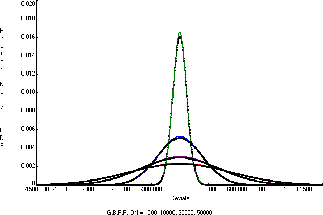 |
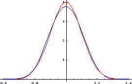
To study this approximation, total distributions were computed for ![]() values of 1000, 10000, 30000, and 50000 DN. Renormalized histograms
were made for each of the N = 1000 distributions described above.
These are shown in Figure 3
as solid lines with colors green, blue, purple, and red, respectively.
Then the pure Gaussian density function was evaluated at the
center of each cell; these values are shown in the figure
as black dots in all cases (the black dots
along each curve are the pure Gaussian values for that
curve's
values of 1000, 10000, 30000, and 50000 DN. Renormalized histograms
were made for each of the N = 1000 distributions described above.
These are shown in Figure 3
as solid lines with colors green, blue, purple, and red, respectively.
Then the pure Gaussian density function was evaluated at the
center of each cell; these values are shown in the figure
as black dots in all cases (the black dots
along each curve are the pure Gaussian values for that
curve's ![]() value). It is obvious from the
figure that the pure Gaussian distributions based on
the average gain are extremely good
approximations to the distributions based on uniform
mixtures over the gain range.
value). It is obvious from the
figure that the pure Gaussian distributions based on
the average gain are extremely good
approximations to the distributions based on uniform
mixtures over the gain range.
This model of the photon noise is applicable even when the gain is not actually varying but is merely unknown and equally likely to be anywhere in the range used. Once a measurement is made, whatever error occurred is always some unknown constant. The distribution of possible values represents the uncertainty in what the error was, not the error itself, which either cannot be known or else could be removed.
As stated earlier, the rules of mathematics and statistics allow one
to formally propagate uncertainties, but in the process one should
be aware of some pitfalls.
A given measurement
![]() undergoes many arithmetic
operations until a final calibrated
value appears out of a pipeline. Some mathematical operations are safe
in the use of the central limit theorem to assume
a normal distribution for the resultant. However, in general, caution
is advised in the invocation of asymptotic normalcy. We
observe that when
undergoes many arithmetic
operations until a final calibrated
value appears out of a pipeline. Some mathematical operations are safe
in the use of the central limit theorem to assume
a normal distribution for the resultant. However, in general, caution
is advised in the invocation of asymptotic normalcy. We
observe that when
![]() , and
, and
![]() then both of the primitive arithmetic operations
then both of the primitive arithmetic operations ![]() and
and ![]() result in
result in
![]() and
and ![]() following a normal distribution. The other two primitive
operations of multiply and divide lead to non-Gaussian results when
following a normal distribution. The other two primitive
operations of multiply and divide lead to non-Gaussian results when
![]() and
and ![]() are calculated.
are calculated.
An interesting case to consider is when we divide two values which we have
reason to believe are each following the Normal distribution. For example,
a value in a pixel is divided by a flat-field to obtain a flattened
image. The pixel value (in the numerator) prior to this operation has
undergone many operations and is seen empirically to follow very closely
a Gaussian distribution. The flat-field has very likely come from the
process of super-medianing or trimmed-averaging of a large number
of independent values, thus it is expected to be a good candidate for
invoking the central limit theorem, and is expected to follow
a Gaussian as well. With these preambles we form the flat-fielded
value ![]() . With a bit of effort one can derive the probability
distribution for
. With a bit of effort one can derive the probability
distribution for ![]() , when
, when
![]() ,
and
,
and
![]() ;
; ![]() has the following form:
has the following form:
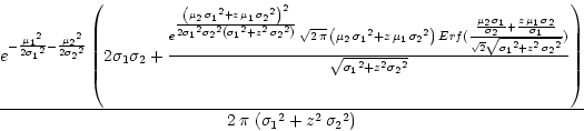
Asymptotically, as
![]() , the distribution becomes Cauchy-like
, the distribution becomes Cauchy-like
It is well known that the Cauchy distribution does not possess first or
higher order moments. Thus we can neither
claim an expected value nor an uncertainty for the flat-fielded result! From
experience we know this to be an absurd proposition; for years people have
used flat-fielded images and have even come up with ``error bars.'' From this
exercise it is clear that assuming Gaussian behavior for the numerator
and denominator (which appeared to be reasonable) can lead to erroneous
conclusions if one attempts to strictly adhere to mathematical
rigor. Instead we must use the rules of plausible reasoning, because
we are dealing with real world scenarios. For one thing, the flat-field
frame is a positive definite quantity, the algorithms that produce the
flat-field must ensure that this is the case. If arithmetic leads to
a non-physical value, that value must be masked appropriately so that
when the result is used in pipeline processing, its non-physical nature
could be communicated. SIRTF calibration pipelines produce such
calibration quality mask files, and use them
for quality assessment (see the step called
CHECKMASK_DP in the example calibration pipeline in
Figure 2.) For another thing, while the denominator (the
flat-field frame) is thought to be Gaussian, this is only in
appearance.
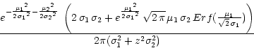
It is possible to come up with a
function that looks very much Gaussian, but in fact has a
compact support (mathematically speaking). This is illustrated in
Figure 4. If we follow the approach of
plausible reasoning and use the lower-peaked curve in
Figure 4 as the distribution of flat-field uncertainties,
then the ratio ![]() will be very well behaved, asymptotically
it will decay rapidly, and will possess moments as well. Following this
approach, since the ratio is now expected to have a second moment, it
is possible to use an equation such as
will be very well behaved, asymptotically
it will decay rapidly, and will possess moments as well. Following this
approach, since the ratio is now expected to have a second moment, it
is possible to use an equation such as
![]() to derive the formal
variance of the ratio (which is very accurate even when the numerator and
denominator have large uncertainties).
to derive the formal
variance of the ratio (which is very accurate even when the numerator and
denominator have large uncertainties).
 |
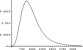
As an application, let us consider again the case of flat fielding.
Suppose that the pixel to be flattened has a value of 1,000 and an
uncertainty of 1.4%, this measurement has a sharp symmetric distribution.
Next suppose the flat-field for that pixel has an uncertainty of
25%,1 the denominator also has a symmetric distribution
(similar to the blue curve in Figure 4). Under this scenario
the probability
distribution for the flat fielded value has the form shown in
Figure 5. The important point to note is that the
distribution is asymmetric (due to the large uncertainty in the
denominator). If a minimum range corresponding to 68% probability
is calculated from the distribution of P(z), the resulting `![]() '
agrees very closely with the expression for
'
agrees very closely with the expression for
![]() that
was discussed earlier.
that
was discussed earlier.
A library of functions dealing with the four primary arithmetic
operations has been developed and used by pipeline modules. For more
complex operations, each module propagates the uncertainty according
to the specific algorithmic form. As example consider detector
non-linearity. The non-linearity coefficient ![]() has been
estimated for each pixel in a calibration pipeline (see
Figure 2); the science pipeline estimates a linearized
DN from the observed DN. The model is simple,
has been
estimated for each pixel in a calibration pipeline (see
Figure 2); the science pipeline estimates a linearized
DN from the observed DN. The model is simple,
![]() . In this case, performing a few reduction steps, the
uncertainty due to the application of the algorithm with the given
. In this case, performing a few reduction steps, the
uncertainty due to the application of the algorithm with the given ![]() becomes
becomes
The input data, ![]() are originally accompanied by uncertainties;
the final uncertainty of the result is obtained by ``rss-ing'' the two
quantities (neglecting first order terms in error expansion, which is
valid in this particular case).
are originally accompanied by uncertainties;
the final uncertainty of the result is obtained by ``rss-ing'' the two
quantities (neglecting first order terms in error expansion, which is
valid in this particular case).
 |
As part of pipeline processing, calibration terms need be applied to the data. In general only a finite number of calibration measurements are performed over a given time period. From those discrete observations, calibration terms must be extended beyond their original domain. Of course with modern instrumentation the builders do their utmost to set up stable and calibratable instruments. The instrument builders count heavily on the power of calibration extension. The process of calibration can fall into two general categories discussed below.
In this scenario, the measured calibration terms are known to be correlated with known control parameters (an instrument builder's dream!) Here, only occasional calibration measurements are performed to verify that the correlation is still valid. The correlation curve is characterized along with uncertainties. At any given time, the calibration term can be ``looked up'' by measuring the control parameter (which could be a frequently sampled House-Keeping parameter) and then using that value to estimate the calibration term and its uncertainty, as illustrated in Figure 6. As stated earlier this is almost dream-like for an instrument builder. With few calibration measurements it is possible to periodically validate the model and continue using a deterministic calibration model.
 |
The case just discussed is usually the exception rather than the rule! More frequently, the dependence of calibration on control parameters is not known well, or there are too many control parameters, each with its own ``seemingly random'' variation. In this case it is difficult, if not impossible, to reach the same level of luxury as in previous section. The purpose of a mission is to maximize science time while staying well calibrated, not to spend most of the time to fully characterize calibration. Thus a few calibration measurements are performed on a routine basis and the principle of ``calibration extension'' is invoked, resulting in a set of calibration rules, for example
Each of these rules leads to different quotes for uncertainties. For example
in the case of fallback, there is no sense of context, thus extend
the uncertainty the same way as the fallback term itself. A more non-trivial
case is when two calibration measurements have been performed at two different
times, and the two calibration products are different without there
being an apparent reason (happens so often!). A calibration rule is then
invoked and the pipelines use a nearest in time value or perhaps an
interpolation between the two. Taking the latter case, in the
absence of evidence to the contrary, assume calibration term changes
continuously from value ![]() at time
at time ![]() to value
to value ![]() at time
at time
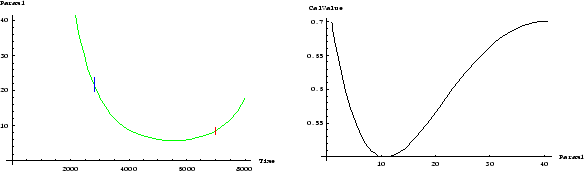
![]() (plausible reasoning). The simplest continuous function is a straight
line. So the calibration extended to time
(plausible reasoning). The simplest continuous function is a straight
line. So the calibration extended to time ![]() is
is
![]() where
where
![]() .
The next issue is what to use for the uncertainty of
.
The next issue is what to use for the uncertainty of ![]() . We stated that
in the absence of information the least costly path from
. We stated that
in the absence of information the least costly path from ![]() at
at ![]() to
to ![]() at
at ![]() appears to be a straight line, but other possibilities
exist as well. A random walk could take us from
appears to be a straight line, but other possibilities
exist as well. A random walk could take us from ![]() at
at ![]() to
to ![]() at
at ![]() also! In fact instruments are known to have drifts, often times
expressible by fractional Brownian Motion (fBM processes). We can postulate
that the variance of
also! In fact instruments are known to have drifts, often times
expressible by fractional Brownian Motion (fBM processes). We can postulate
that the variance of ![]() used at time t is
used at time t is
![]() , where
, where
![]() , similarly for
, similarly for ![]() . This
results in the growth of uncertainty in the interpolation scheme that
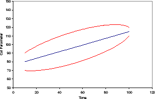
is seen in Figure 7. Plausible reasoning has led to
a growth of uncertainty as we go farther away from the epoch of
calibration measurement.
. This
results in the growth of uncertainty in the interpolation scheme that
is seen in Figure 7. Plausible reasoning has led to
a growth of uncertainty as we go farther away from the epoch of
calibration measurement.
 |
Moshir, M. 2001, in ASP Conf. Ser., Vol. 281, Astronomical Data Analysis Software and Systems XI, ed. David A. Bohlender, Daniel Durand and T. H. Handley (San Francisco: ASP), 336
Fang, F. et al. 2003, this volume, 253
Moshir, M. et al. 1992, Explanatory Supplement to the IRAS Faint Source Survey, Version2, JPL D-10015 8/92 (Pasadena:JPL)
Masci, F. et al. 2003, this volume, 391