Next: A New IRAF Catalog Access Tool for Astrometry
Up: Iraf Packages
Previous: A Spectroscopy Exposure Time Calculator for IRAF
Table of Contents -
Subject Index -
Author Index -
PS reprint -
Acosta-Pulido, J. A. 2000, in ASP Conf. Ser., Vol. 216, Astronomical Data
Analysis Software and Systems IX, eds. N. Manset, C. Veillet, D. Crabtree (San Francisco: ASP), 663
TwoFitlines: An Spectrum and Line Analysis Tool
J. A. Acosta-Pulido
Institituto Astrofísica de Canarias, 38200 La Laguna - SPAIN
Abstract:
Twofitlines is a tool developed within IRAF, optimized to be used with
data containing multiple spectra along the spatial axis of the detector.
A given spectral feature can be decomposed in one or several
Gaussian components.
The results are obtained in handy graphical and text formats.
The error in the fitted parameters is estimated by successive fits to
Montecarlo simulated spectra.
An extra capability allows to measure useful asymmetry parameters for
non-resolved spectral features.
Twofitlines is a task developed to facilitate the analysis of spectroscopic
data, containing multiple spectra along the spatial axis of the detector. These
type of data are produced by longslit, multislits or fiber spectrographs.
The basic requirements to build such tool were:
- A given spectral feature can be modeled using one or more
components (currently only Gaussian profiles are available),
- The fitting model should be easily and interactively configurable,
- It should keep memory of the best fitting model when moving across
the spectra,
- The continuum can be modeled separately from the spectral features,
which is especially important when measuring faint emission or
absorption lines,
- Close spectral features could be modeled simultaneously.
The variation of Gaussian parameters for the various lines can be constrained
in different ways,
- It should be used in a similar way in both interactive and background
modes.
There exist tools in IRAF which allows to measure spectral line features using
different profiles, for instance splot, fitprofs, and specfit.
These three
tasks cover most of the above requirements, although each of them has its own
limitations. Some time ago, we decided to take what was considered the best
from each task and put it together into a unique task. The final result
closely resembles those mentioned tasks.
The programming language is SPP, and it is structured as
a mini-package in IRAF called twofitlines,
although the task actually doing the work is called fitlines.
The tool is available at the ftp address
ftp://ftp.iac.es/pub/users/jacosta/twofitlines.tar.gz.
Spectra can be read from images in a variety of IRAF formats for spectroscopic
data.The basic input parameters are a fitting region, a
list of initial positions and widths, plus some constrains.
The program can be used in both interactive or background modes.
The main features of fitlines are described below:
- 1.
- Two minimization algorithms can be selected, Levenberg-Marquadt
or Simplex;
- 2.
- The uncertainty of model parameters is determined by a number
of repeated fits to simulated data in the following way:
- i.
- An specified model with a given number of components is
fit to the selected spectral region, obtaining the best fitting model
parameters;
- ii.
- Random Gaussian noise is added to each pixel value as
computed from the best fitting model. Two type of noises can be added:
the noise amplitude is uniform along the spectrum, or based in Poisson
statistics;
- iii.
- A new model is fitted to the simulated spectrum, taking as starting
values those recently obtained. The new parameter models are saved
temporarily. After a number of tries the error of each fitting
parameter is computed as the standard deviation.
- 3.
- Output results in non-interactive mode can be saved in
graphical and text formats for later inspection;
- 4.
- Initial values for a fit can be read from a database file.
This file can be manually edited or directly created from a successful fit.
This is very useful for non-interactive processing of large amount of data.
Figure 1:
List of available parameters in interactive modes.
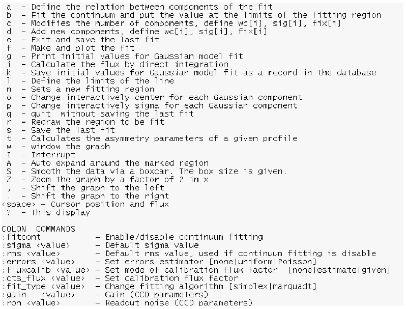 |
A variety of commands are available in interactive mode, which allow to perform
any model fit, output the results and saving the parameters to be used as
initial values for next fitting operations (see Figure 1).
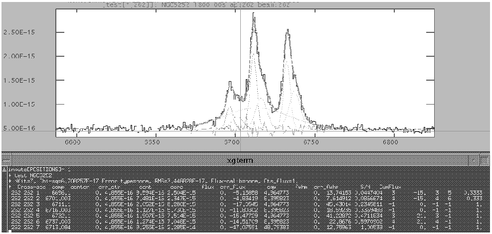
The results of the fitting process are the computed parameters
(line center, amplitude and width), the flux and the equivalent width
for each component.
The flux included within the limits of the selected spectral feature
is also computed by simply adding each spectrum bin after
continuum subtraction.
The goodness of the fit can be easily assessed from the comparison of the total
flux which results from the addition of all model components and the direct
sum just mentioned. The reliability of each model component is also inferred
from the S/N ratio, i.e. the line peak to the continuum noise ratio
(see Figure 2).
Sometimes it is worth to set relationships in between some components
parameters, e.g. if two
emission lines are expected to come from the same region the width
could be the same, or to fix the ratio between intensity of line sets,
give same center offsets to line sets.
One of the remarkable features of fitlines is the capability to set
model fit constrains in a
flexible and interactive way. At the moment there are four
ways of setting constrains for each parameter group: (1) all vary
freely; (2) all are fixed to the initial values;
(3) only the value
for one component varies and the others are offset/scaled by a the initial
values; and (4) for each component one parameter can be set to vary
independently, fixed to a specific value or to be tight to another component.
An example of the last type is presented in Figure 2. The
emission line complex H +[NII]
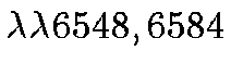 is modeled
including physical constrains. There are two components per line of similar
width plus a broad one for H.
The kinematically coupled components obey the following conditions:
same line width, constant wavelength
offset, and constant flux ratio for [NII]
.
is modeled
including physical constrains. There are two components per line of similar
width plus a broad one for H.
The kinematically coupled components obey the following conditions:
same line width, constant wavelength
offset, and constant flux ratio for [NII]
.
Spectral features show in many occasions complex line profiles, or relatively
smooth asymmetric profiles which reflect the complex internal velocity field
of the emission source or the poor spectral or spatial resolution of our
spectra. In these cases the decomposition into a number of Gaussian
components does not produce a set of meaningful parameters.
More general approaches have been proposed
(Whittle 1985; Heckman et al. 1981), such as measuring the width,
the center and asymmetry at different heights of the profile.
The two above parameterizations are included in the program fitlines and can be
applied to any 1-D or 2-D spectrum.
References
Heckman, T. M., Butcher, H. R., Miley, G. K., & van Breugel,
W. J. M 1981, ApJ, 247, 403
Whittle, M. 1985, MNRAS, 213, 1
© Copyright 2000 Astronomical Society of the Pacific, 390 Ashton Avenue, San Francisco, California 94112, USA
Next: A New IRAF Catalog Access Tool for Astrometry
Up: Iraf Packages
Previous: A Spectroscopy Exposure Time Calculator for IRAF
Table of Contents -
Subject Index -
Author Index -
PS reprint -
adass@cfht.hawaii.edu