P. Ballester
European Southern Observatory,
Karl-Schwarzschild-Str. 2, D-85748 Garching, Germany
Keywords: spectroscopy, Hough transform, wavelet transform, robust regression, echelle, wavelength calibration
Classical statistical techniques usually lack the ability to reject outliers which appear in real data, resulting from measurement errors, mixed distributions, noise, etc. Different methods offer inherent robust properties in the presence of contamination. The application of robust methods to the domain of spectral data analysis is reviewed in this paper. A short introduction to robust regression by Least-Median of Squares is presented in Section 2. This algorithm is applied to the determination of echelle dispersion relations. Section 3 is an excerpt from a recently published article (Ballester 1994) related to the Hough transform and its application to echelle order detection and automated arc line identification. Wavelet transform can be useful in complementing robust techniques for multiresolution analysis, and Section 4 presents an application of the Mexican hat transform to the detection of spectral features.
The sensitivity of least-squares (LS) regression to outliers is a traditional problem in data analysis, and as an alternative Rousseeuw (1987) introduced the Least Median of Squares (LMS) which consists of minimizing the term:

This minimization cannot be obtained analytically and
therefore requires repeated evaluations for different subsamples
of size p drawn from the n observations. A complete trial
would require  evaluations which would rapidly become
impracticable for large n and p values. Rousseeuw & Leroy
(1987) determined the minimum number m of subsamples required to obtain a
given probability
  of drawing at least one subsample
containing only good observations from a sample containing a
fraction
  of outliers. By requiring
  to
be sufficiently close to 1 (e.g 0.95 or 0.99), m
can be determined for given values of p and
  :
:

The smallest fraction  of contamination that can
cause the estimator to deviate arbitrarily from the estimate
performed on the uncontaminated sample is called the breakdown
point of the estimator. In the case of the LS estimator, only one
outlier is sufficient to make the fitted parameters deviate
arbitrarily from the expected value, therefore the breakdown point
of LS is 0%. The LMS-based Reweighted Least Square (RLS)
corresponds geometrically to finding the narrowest strip covering
half of the observations. The breakdown point of the RLS is 50%.
Most the other robust estimators do not attain a breakdown point of
30% (Rousseeuw & Leroy 1987). In the following sections
of this paper, the applications have been realized using the PROGRESS
algorithm available from the Statlib statistical library (e-mail:
statlib@lib.stat.cmu.edu).
Wavelength calibration using an arc lamp exposure is a basic step in spectral calibration, usually requiring a careful analysis of errors and selection of lines, especially in echelle spectroscopy where arc spectra containing several hundreds of lines are commonly found. Several problems occur when using standard polynomial regression:
Robust regression is an adapted method to take care of these
problems. By combining Hough transform based automated
arc line identification and robust regression, it is possible
to perform an automated calibration,
providing as information the central wavelength
and the average dispersion in a single order. This first
estimate is refined by Hough transform cross-matching
and extended to the complete spectrum using the echelle relation
 . However the accuracy of this relation
is limited by several factors: in particular, optical misalignments
occurring between echelle grating, cross-disperser, and detector. In
the first iteration
the unknown rotation angle is introduced into the error model of the
echelle relation. Lines are then identified by a
robust regression based iterative loop.

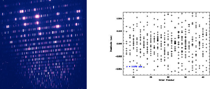
Figure: Th-Ar exposure obtained with the EMMI spectrograph at La Silla
observatory and figure of residuals.
Original PostScript figures
(650 kB),
(40 kB)
Figure 1 shows the calibration of a Th-Ar exposure taken with
the EMMI spectrograph at La Silla observatory. The wavelength
range covered is 380--940nm over 24 orders. The combination
of arc line identification by Hough transform and robust regression
allows to perform the calibration with the only information of
central wavelength (679nm  50 pixels), average dispersion
(0.03nmpixel
 30%)
and absolute order number (24) for the relative order 18.
The method requires no instrument dependent knowledge and allows
for a relatively large inaccuracy of the initial solution. The figure
of residuals shows a final accuracy of about
  pixel rms.
The Th-Ar line catalog was
provided by H. Hensberge and corrected for line
blending (De Cuyper & Hensberge 1995).
A description of the Hough transform and its astrophysical applications can be found in Ballester (1994) and Ragazonni & Barbieri (1994). For the application of the HT to the detection of echelle orders, we use a representation of the HT assuming no preliminary segmentation of the image, since the sought-for features are brighter than the background. Accumulating a function of the intensity makes it possible to detect the orders by order of brightness.
The identification of arc lines consists of associating a list of line
positions in pixel space with a list of reference wavelengths. The principle
of the method is to perform all possible associations in a pixel-wavelength
space. A three-dimensional HT allows us to detect, within a given range of
central wavelength and average dispersion, the non-linear dispersion relation
maximizing the number of associations. In the general case, the maximum is
searched for in a cube of the Hough space, providing the parameters
 of the dispersion relation:
 . Usually the
simplification
  makes it possible to use a two-dimensional HT.
The wavelet transform has been widely described
(e.g., Starck, Murtagh, & Bijaoui 1995) and consists of the convolution product of
a function with an analyzing wavelet. By choosing a wavelet which
is the second derivative of a smoothing
function, the wavelet coefficients become proportional to the
second derivative of the smoothed signal.
The Mexican hat transform involves the wavelet:
 which is the second derivative of a Gaussian.
Since the continuum of a spectrum varies smoothly, its second
derivative will show increased values at the position of sharper
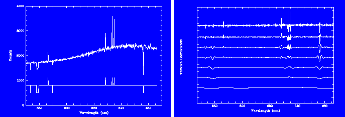
spectral features. Figure 2 shows the Mexican hat transform
of a spectrum presenting emission features, as well as absorption
lines, of different widths. The wavelet coefficients become maximum
(in absolute value) at different scales depending on the spatial
extension of the features. The Mexican hat transform can be used to
generate a multiresolution mask of the spectral features. The
transformation applied to the wavelet coefficients at the different
scales includes segmentation, generation of windows, and
multiresolution recombination using a coarse-to-fine approach.
After segmentation at each scale, the coefficients
are compared between successive scales. The process starts from the
largest scale and a feature will be retained at the next scale if its
associated wavelet coefficients are larger. After recombination
the mask is binarized and provides a schematic representation of the
spectrum, providing the positions of the continuum and of the features.

Figure: Spectrum of a standard star and associated binary mask
(after scaling and translation), and dyadic Mexican hat
transform of the above spectrum decomposed
on 7 scales. The coefficients of the sharp positive features are
concentrated at small scales.
Coefficients of the absorption lines are maximized at different scales,
depending on their spatial extension.
Original PostScript figures
(24 kB),
(42 kB)
I would like to thank P. Grosbøl, H. Hensberge, F. Murtagh, and J. L. Starck for helpful discussions.
De Cuyper J. P., & Hensberge H. 1995, ![]()
Ragazzoni R., & Barbieri C. 1994, PASP, 106, 683
Rousseeuw P. J., & Leroy A. M. 1987, Robust Regression and Outlier Detection (New York, Wiley)
Starck J. L., Murtagh, F., & Bijaoui, A. 1995, ![]()